方程 $z^n=1\quad (n=1,2,3,\cdots)$ 的复数根 $z$ 为 $n$ 次单位根[1]
下面求解该方程。
已知欧拉公式[2]
$$e^{i\pi}+1=0$$
则:
$$(e^{i\pi})^2=(-1)^2$$
$$e^{2i\pi}=1$$
两边作 $k$ 次方:
$$e^{i2k\pi}=1$$
再取 $n$ 次根,得:
$$\sqrt[n]{1}=e^{i2\pi \frac{k}{n}}=\cos 2\pi \frac{k}{n}+i\sin 2\pi \frac{k}{n}$$
由三角函数的周期性易知,其根有 $n$ 个,分别是 $k$ 取 $0,1,2,\cdots ,n-1$
即,单位的 $n$ 次根有 $n$ 个:
$$e^{\frac{2\pi ki}{n}} \quad (k=0,1,2,\cdots ,n-1)$$
单位的 $n$ 次根以乘法构成 $n$ 阶循环群,生成元是 $n$ 次本原单位根$n$ 次本原单位根是 $e^{\frac{2\pi ki}{n}}$ ,其中 $k$ 和 $n$ 互质。因此由欧拉函数定义,$n$ 次本原单位根数目为欧拉函数 $\varphi (n)$ .
例子:
一次单位根有一个:$1$
二次单位根有两个:$+1$ 和 $-1$ ,只有 $-1$ 是本原根
三次单位根是(除 1 外都是本原根):
$$\{1,\frac{-1+\sqrt{3}i}{2},\frac{-1-\sqrt{3}i}{2}\}$$
- 四次单位根是:
$\{1,+i,-1,-i\}$ ,其中
$+i$ 和
$-i$ 是本原根
当 $n$ 不小于 2 时,n 次单位根总和为 0 .
$$\sum\limits_{k=0}^{n-1}e^{\frac{2\pi ki}{n}}=\frac{e^{\frac{2\pi kni}{n}}-1}{e^{\frac{2\pi i}{n}}-1}=\frac{1-1}{e^{\frac{2\pi i}{n}}-1}=0$$
该结果在复平面上是显然的。
部分内容参考自视频 The Fast Fourier Transform (FFT): Most Ingenious Algorithm Ever? 只有生肉,没有找到较好的翻译版本。因此使用了部分英语表述。这个视频在记法上有一些蛊惑人心的地方,我就按照自己的习惯来了。
问题引入:我们试图计算两个多项式的乘积。朴素的做法是使用乘法的分配律在 $O(n^2)$ 时间内完成。现在需要寻找更高效的算法。
为此引入 Polynomial Representation 的另一种方法:value representation.
Coefficient Representation :
$$P(x)=p_0+p_1x+p_2x^2+\cdots p_dx^d$$
$$\begin{matrix} \underbrace{[p_0,p_1,\cdots ,p_d]} \\ {\scriptstyle\text{Coefficient Representation}} \end{matrix}$$
Value Representation :
$$\begin{matrix} \underbrace{\{(x_0,P(x_0)),(x_1,P(x_1)),\cdots ,(x_d,P(x_d))\}} \\ {\scriptstyle\text{Value Representation}} \end{matrix}$$
两者之间的关系:
$(d+1)$ points uniquely define a degree $d$ polynomial.
$e.g.$
$$\{(-1,0),(0,1),(1,0),(2,1)\}$$
Corresponds to
$$P(x)=\frac{2}{3}x^3-x^2-\frac{2}{3}x+1$$
$Proof.$
$$\begin{bmatrix}
P(x_0) \\
P(x_1) \\
\vdots \\
P(x_d)
\end{bmatrix}=\begin{bmatrix}
1 & x_0 & x_0^2 & \cdots & x_0^d \\
1 & x_1 & x_1^2 & \cdots & x_1^d \\
\vdots & \vdots & \vdots & \ddots & \vdots \\
1 & x_d &x_d^2 & \cdots & x_d^d
\end{bmatrix}\begin{bmatrix}
p_0 \\
p_1 \\
\vdots \\
p_d
\end{bmatrix}$$
Clearly, the determinant of the matrix above is the Vandermonde determinant.
Since the chosen values of $x_i (i=0,1,2,\cdots ,d)$ are distinct from each other, the Vandermonde determinant is non-zero.
$$\det \begin{pmatrix}\begin{bmatrix}
1 & x_0 & x_0^2 & \cdots & x_0^d \\
1 & x_1 & x_1^2 & \cdots & x_1^d \\
\vdots & \vdots & \vdots & \ddots & \vdots \\
1 & x_d &x_d^2 & \cdots & x_d^d
\end{bmatrix}\end{pmatrix}=\prod_{0\leqslant j<i\leqslant d}(x_i-x_j)\neq 0$$
Therefore, the matrix is invertible, and the equation has a unique solution.
Hence, a bijection is established between the value representation and the coefficient representation of the polynomial through this matrix. $(d+1)$ points uniquely define a degree $d$ polynomial.
■
有了两个多项式的 value representation ,就可以很容易地计算出这两个多项式的乘积的 value representation.
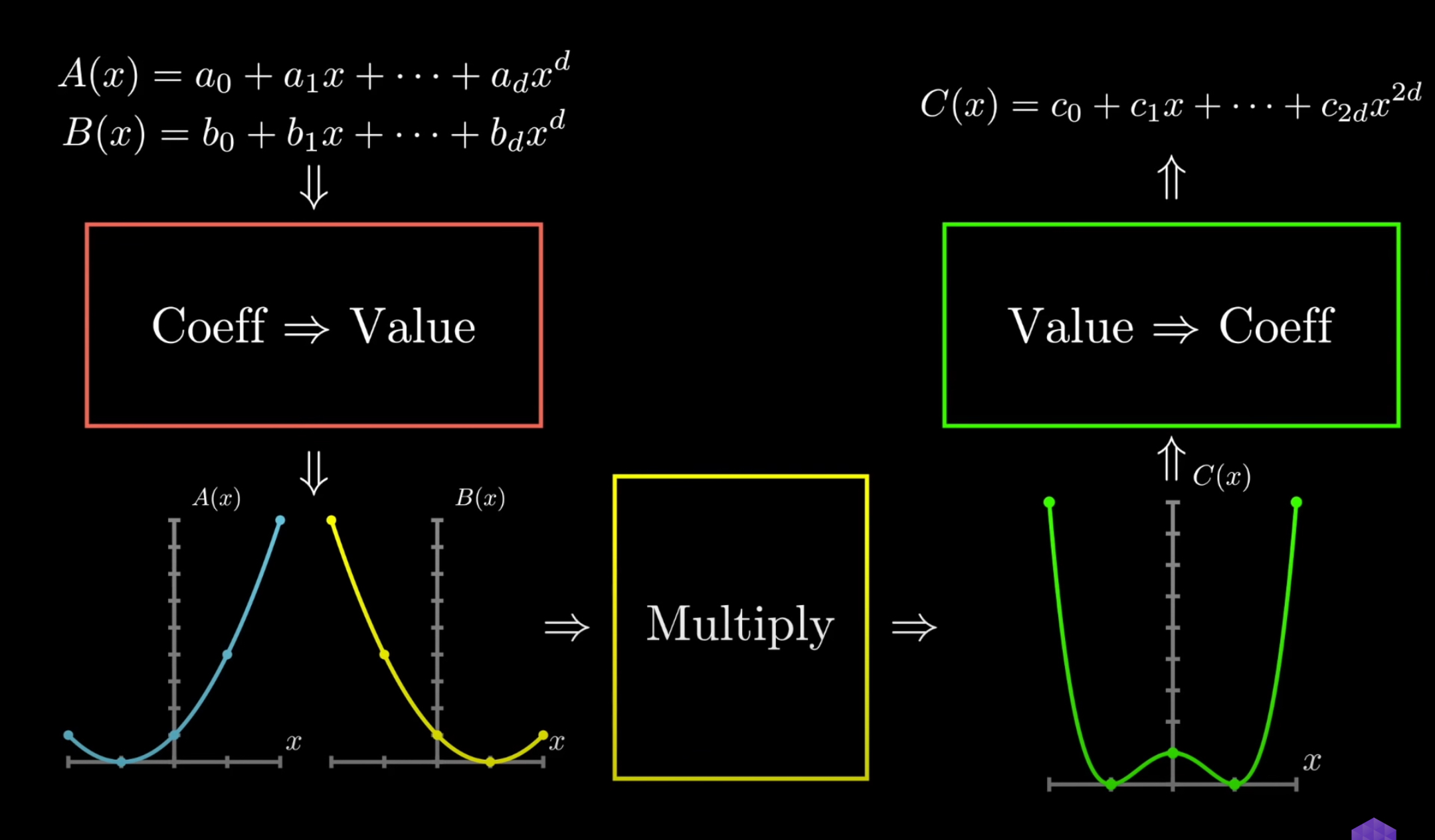
整个过程的大致思路如下:
41-1.jpg 首先考虑 Coeff 到 Value 的转换。
我们尝试计算 n-1 次多项式 $P(x)$ 在
$$x=\pm x_1,\pm x_2,\cdots ,\pm x_{n/2}$$
处的值,寻找能减少计算量的思路。
将 $P(x)$ 按项的次数奇偶分类:
$$P(x)=P_e(x^2)+xP_o(x^2)$$
得到 $P_e(x)$ 和 $P_o(x)$ . 于是:
$$P(\pm a)=P_e(a^2)\pm aP_o(a^2)$$
于是问题转化为求 $P_e(x)$ 和 $P_o(x)$ 在 $a^2$ 处的值,这个过程似乎可以递归地进行。而且这两个多项式的次数比原来下降了一半。看起来很 nice .
而问题是,进入第二层递归时,我们的采样点就不是相反数对了。递归失败。
以上尝试给出了有益的思路,接下来为了制造相反数对,考虑将数域拓展到复数。
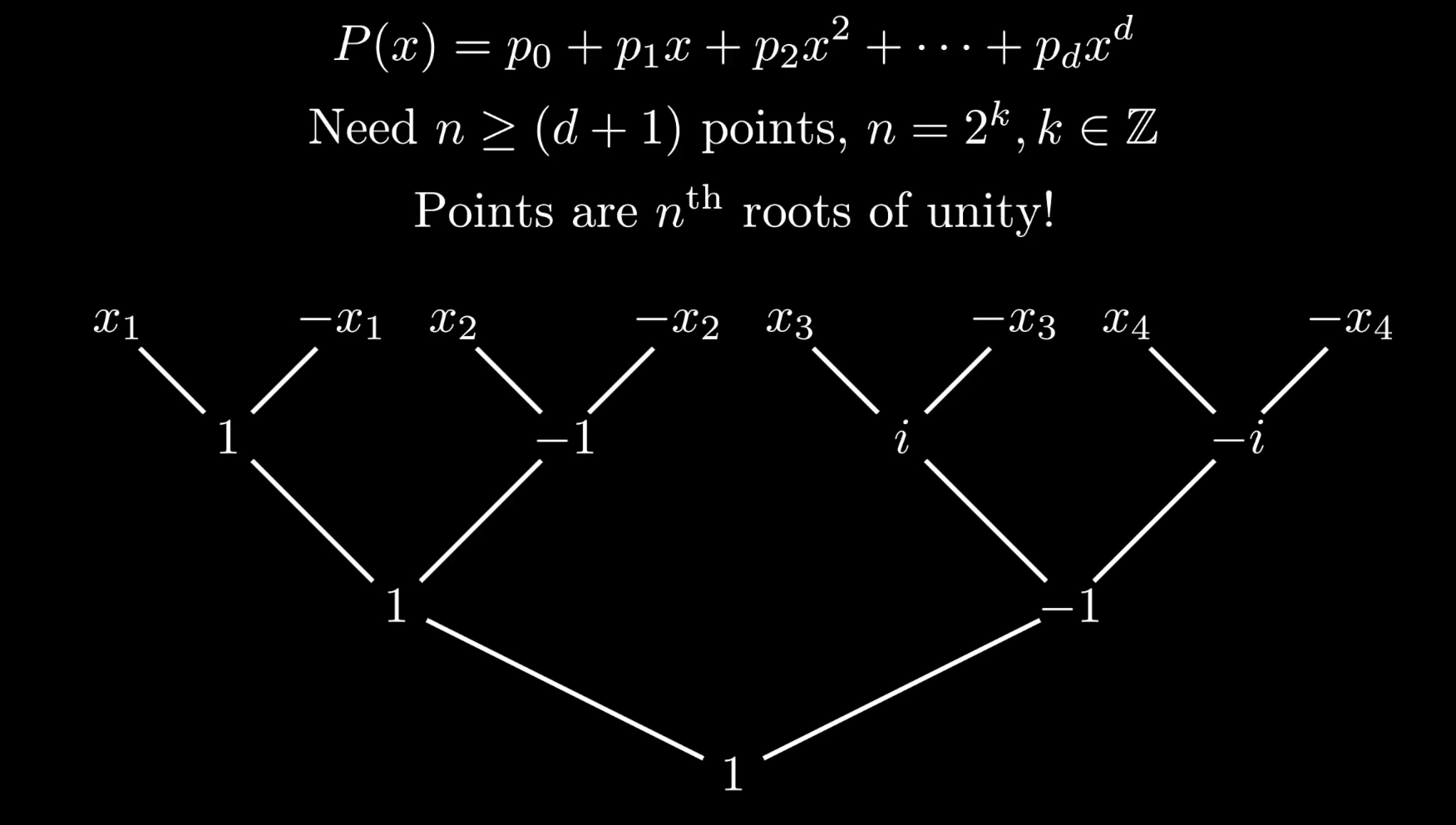
在下图中,任一节点的值的平方等于父节点的值:
41-2.png 满足我们想要的性质。注意这里为方便原理展示对采样点数目 $n$ 作了限制:$n=2^k,k\in \mathbb{N}$ . 同时这也是对多项式次数的限制。
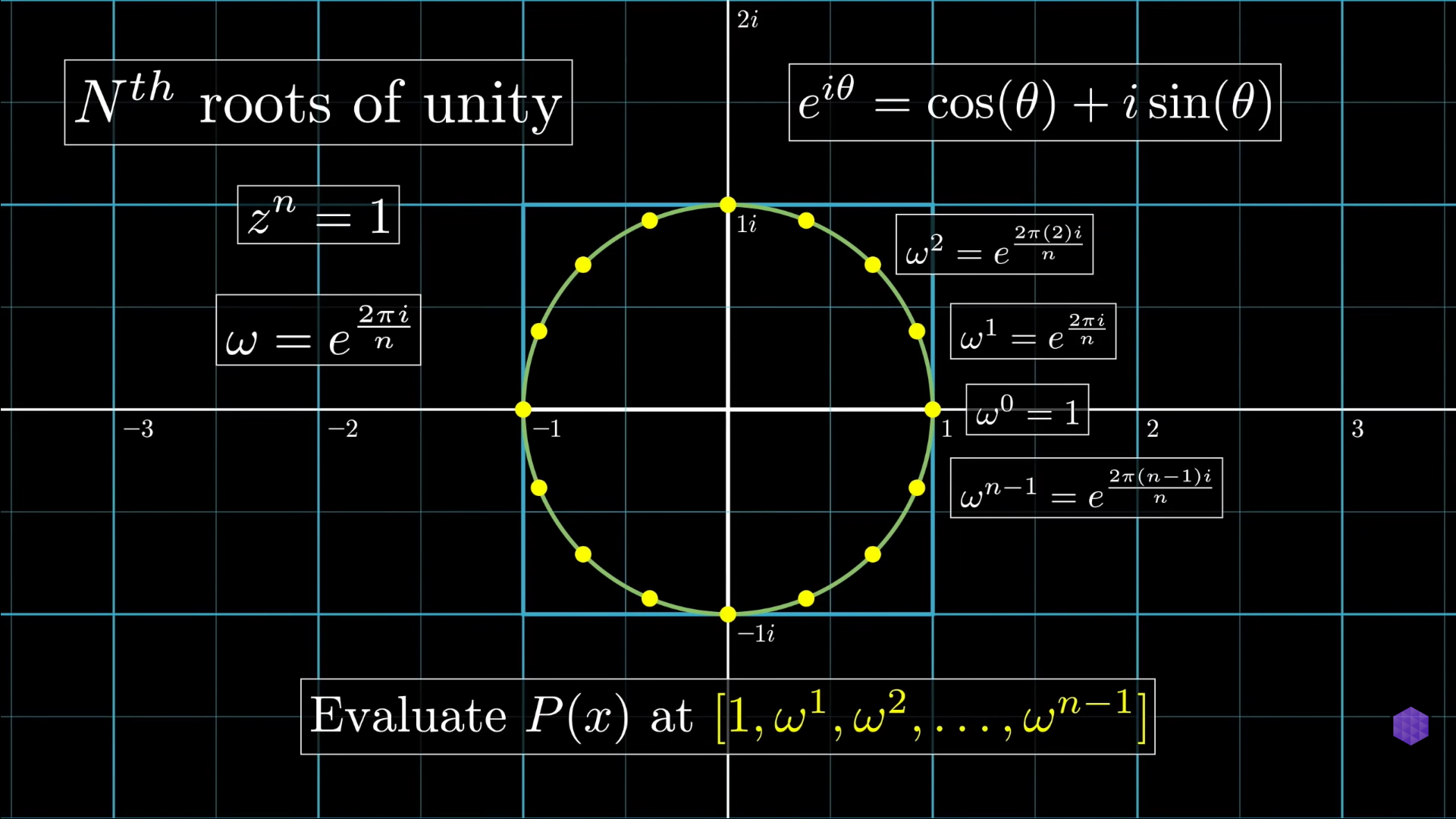
依据在前置知识中的结论,单位根在复平面中如下所示:
41-3.png 并且,由相关性质,可以得到相反数对:
41-4.png $$\omega ^{j+n/2}=-\omega ^j$$
下面总结一下算法的流程。
为求出 n-1 次多项式 $P(x)$ 的 value representation ,需要计算其在
$$x=\omega ^0,\omega ^1,\cdots ,\omega ^{n-1} \quad | \quad \omega =e^{\frac{2\pi i}{n}}$$
处的值。为了减少计算量,将 $P(x)$ 按项的次数奇偶分类:
$$P(x)=P_e(x^2)+xP_o(x^2)$$
由是发现需要求解 $P_e(x)$ 和 $P_o(x)$ 在
$$\omega ^0,\omega ^2,\omega ^4, \cdots ,\omega ^{n-2}$$
处的值。这个过程可以递归地完成。
注意这里就是原视频蛊惑人心的地方,UP主在记法上的不严谨可能会导致理解上的困难。$P_e(x)$ 和 $P_o(x)$ 是将公式 $P(x)=P_e(x^2)+xP_o(x^2)$ 右侧的多项式 $P_e(x^2)$ 和 $P_o(x^2)$ 看作 $x^2$ 的函数用 $x$ 改写得到的。
假设递归成功,就得到了 $P_e(x)$ 和 $P_o(x)$ 的 value representation . 记数组(从 0 开始编号):
$$y_e[...]=[P_e(\omega ^0),P_e(\omega ^2),\cdots ,P_e(\omega ^{n-2})]$$
$$y_o[...]=[P_o(\omega ^0),P_o(\omega ^2),\cdots ,P_o(\omega ^{n-2})]$$
现在要做的是,由此得到原来的多项式的 value representation .
在上面得到的公式
$$P(\pm a)=P_e(a^2)\pm aP_o(a^2)$$
中,令 $a=\omega ^j$ 得:
$$P(\pm \omega ^j)=P_e(\omega ^{2j})\pm \omega ^jP_o(\omega ^{2j})$$
再由 $\omega ^{j+n/2}=-\omega ^j$ 得:
$$P(\omega ^j)=P_e(\omega ^{2j})+ \omega ^jP_o(\omega ^{2j})$$
$$P(\omega ^{j+n/2})=P_e(\omega ^{2j})- \omega ^jP_o(\omega ^{2j})$$
$$j\in \{0,1,\cdots ,\frac{n}{2}-1 \}$$
又因为
$$y_e[j]=P_e(\omega ^{2j})$$
$$y_o[j]=P_o(\omega ^{2j})$$
于是
$$P(\omega ^j)=y_e[j]+ \omega ^jy_o[j]$$
$$P(\omega ^{j+n/2})=y_e[j]- \omega ^jy_o[j]$$
$$j\in \{0,1,\cdots ,\frac{n}{2}-1 \}$$
最后返回该层多项式的 value representation 即可。
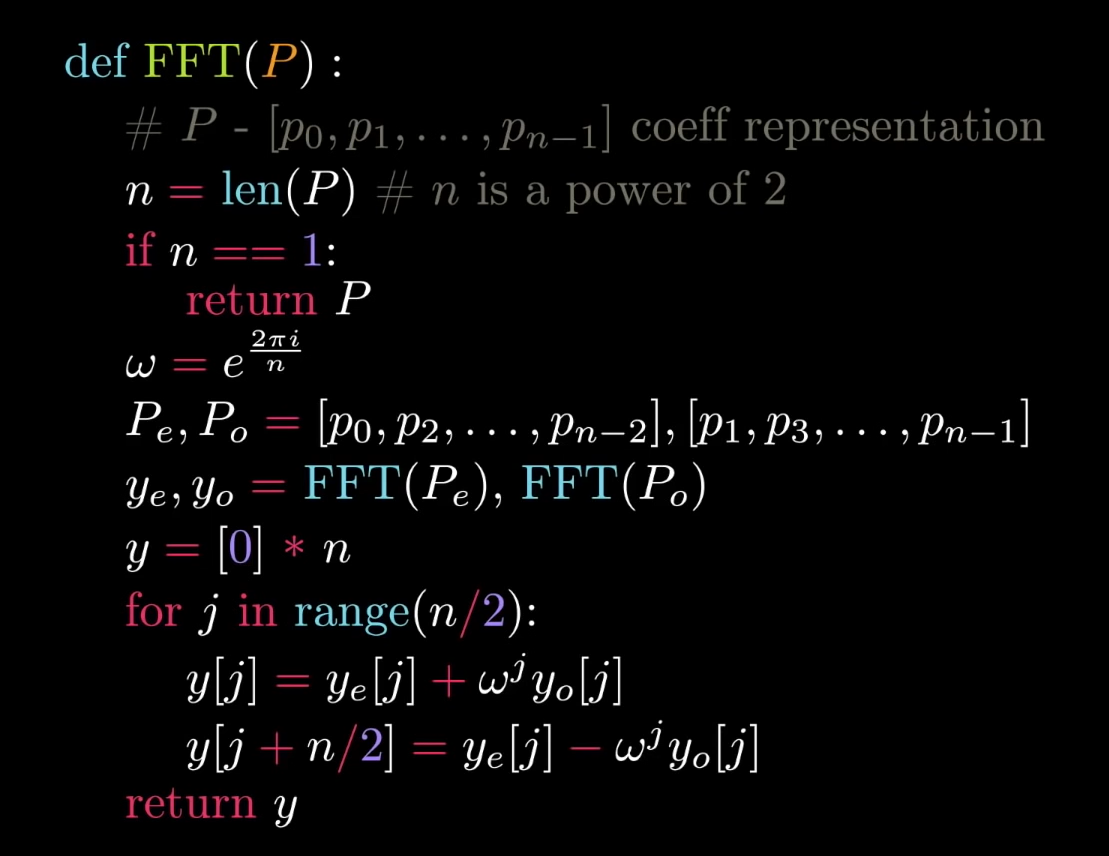
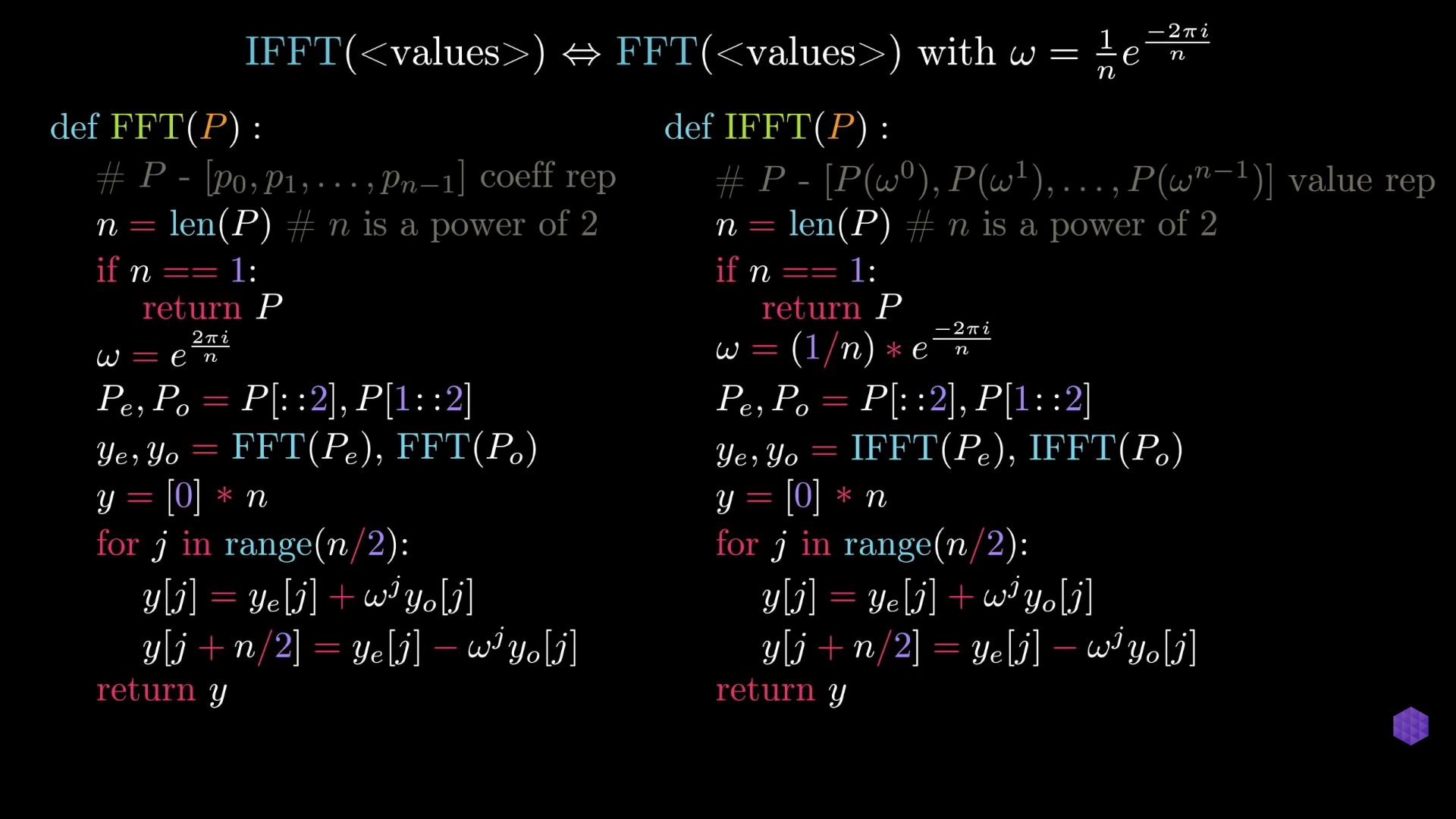
伪代码如下:
41-5.png 返回看下图 41-1.jpg ,还需要完成 Value 到 Coeff 的转换。
在之前的式子中:
$$\begin{bmatrix}
P(x_0) \\
P(x_1) \\
\vdots \\
P(x_{n-1})
\end{bmatrix}=\begin{bmatrix}
1 & x_0 & x_0^2 & \cdots & x_0^{n-1} \\
1 & x_1 & x_1^2 & \cdots & x_1^{n-1} \\
\vdots & \vdots & \vdots & \ddots & \vdots \\
1 & x_{n-1} &x_{n-1}^2 & \cdots & x_{n-1}^{n-1}
\end{bmatrix}\begin{bmatrix}
p_0 \\
p_1 \\
\vdots \\
p_{n-1}
\end{bmatrix}$$
令 $x_k=\omega ^k\quad \mathrm{where}\quad \omega =e^{\frac{2\pi i}{n}}$
$$\begin{bmatrix}
P(\omega ^0) \\
P(\omega ^1) \\
P(\omega ^2) \\
\vdots \\
P(\omega ^{n-1})
\end{bmatrix}=\begin{bmatrix}
1 & 1 & 1 & \cdots & 1 \\
1 & \omega & \omega ^2 & \cdots & \omega ^{n-1} \\
1 & \omega ^2 & \omega ^4 & \cdots & \omega ^{2(n-1)} \\
\vdots & \vdots & \vdots & \ddots & \vdots \\
1 & \omega ^{n-1} & \omega ^{2(n-1)} & \cdots & \omega ^{(n-1)(n-1)}
\end{bmatrix}\begin{bmatrix}
p_0 \\
p_1 \\
p_2 \\
\vdots \\
p_{n-1}
\end{bmatrix}$$
上式中的矩阵被称为 Discrete Fourier Transform (DFT) matrix
$$\begin{bmatrix}
p_0 \\
p_1 \\
p_2 \\
\vdots \\
p_{n-1}
\end{bmatrix}=\begin{bmatrix}
1 & 1 & 1 & \cdots & 1 \\
1 & \omega & \omega ^2 & \cdots & \omega ^{n-1} \\
1 & \omega ^2 & \omega ^4 & \cdots & \omega ^{2(n-1)} \\
\vdots & \vdots & \vdots & \ddots & \vdots \\
1 & \omega ^{n-1} & \omega ^{2(n-1)} & \cdots & \omega ^{(n-1)(n-1)}
\end{bmatrix}^{-1}\begin{bmatrix}
P(\omega ^0) \\
P(\omega ^1) \\
P(\omega ^2) \\
\vdots \\
P(\omega ^{n-1})
\end{bmatrix}$$
求出矩阵的逆:
$$\begin{bmatrix}
p_0 \\
p_1 \\
p_2 \\
\vdots \\
p_{n-1}
\end{bmatrix}=\frac{1}{n}\begin{bmatrix}
1 & 1 & 1 & \cdots & 1 \\
1 & \omega ^{-1} & \omega ^{-2} & \cdots & \omega ^{-(n-1)} \\
1 & \omega ^{-2} & \omega ^{-4} & \cdots & \omega ^{-2(n-1)} \\
\vdots & \vdots & \vdots & \ddots & \vdots \\
1 & \omega ^{-(n-1)} & \omega ^{-2(n-1)} & \cdots & \omega ^{-(n-1)(n-1)}
\end{bmatrix}\begin{bmatrix}
P(\omega ^0) \\
P(\omega ^1) \\
P(\omega ^2) \\
\vdots \\
P(\omega ^{n-1})
\end{bmatrix}$$
这个时候简直是 amazing 啊,上面这个矩阵和之前的那个矩阵形式几乎一样,那么我们在代码上只需要少量改动。
Every $\omega$ in original matrix is now $\frac{1}{n}\omega ^{-1}$ .
伪代码:
41-6.png 至此已分析完算法的原理部分。
[1] 维基百科 - 单位根 (已备份)
[2] SeriesNote 函数的幂级数展开式的应用